Monte Carlo Dropout for Semantic Segmentation on MUAD

This tutorial demonstrates how to train a segmentation model on the MUAD dataset using TorchUncertainty. MUAD is a synthetic dataset designed for evaluating autonomous driving under diverse uncertainties. It includes 10,413 images across training, validation, and test sets, featuring adverse weather, lighting conditions, and out-of-distribution (OOD) objects. The dataset supports tasks like semantic segmentation, depth estimation, and object detection.

For details and access, visit the MUAD Website.

1. Loading the utilities

First, we load the following utilities from TorchUncertainty:

• the TUTrainer which mostly handles the link with the hardware (accelerators, precision, etc)

• the segmentation training & evaluation routine from torch_uncertainty.routines

• the datamodule handling dataloaders: MUADDataModule from torch_uncertainty.datamodules

• the model: small_unet from torch_uncertainty.models.segmentation.unet

• the MC Dropout wrapper from torch_uncertainty.models

import matplotlib.pyplot as plt
import torch
import torchvision.transforms.v2.functional as F
from huggingface_hub import hf_hub_download
from torch import optim
from torch.optim import lr_scheduler
from torchvision import tv_tensors
from torchvision.transforms import v2
from torchvision.utils import draw_segmentation_masks

from torch_uncertainty import TUTrainer
from torch_uncertainty.datamodules.segmentation import MUADDataModule
from torch_uncertainty.models import mc_dropout
from torch_uncertainty.models.segmentation.unet import small_unet
from torch_uncertainty.routines import SegmentationRoutine

2. Initializing the DataModule

muad_mean = MUADDataModule.mean
muad_std = MUADDataModule.std

train_transform = v2.Compose(
    [
        v2.Resize(size=(256, 512), antialias=True),
        v2.RandomHorizontalFlip(),
        v2.ToDtype(
            dtype={
                tv_tensors.Image: torch.float32,
                tv_tensors.Mask: torch.int64,
                "others": None,
            },
            scale=True,
        ),
        v2.Normalize(mean=muad_mean, std=muad_std),
    ]
)

test_transform = v2.Compose(
    [
        v2.Resize(size=(256, 512), antialias=True),
        v2.ToDtype(
            dtype={
                tv_tensors.Image: torch.float32,
                tv_tensors.Mask: torch.int64,
                "others": None,
            },
            scale=True,
        ),
        v2.Normalize(mean=muad_mean, std=muad_std),
    ]
)

# datamodule providing the dataloaders to the trainer
datamodule = MUADDataModule(
    root="./data",
    batch_size=10,
    version="small",
    train_transform=train_transform,
    test_transform=test_transform,
    num_workers=4,
)
datamodule.prepare_data()
datamodule.setup("fit")

Visualize a validation input sample (and RGB image)

# Undo normalization on the image and convert to uint8.
img, tgt = datamodule.train[0]
t_muad_mean = torch.tensor(muad_mean, device=img.device)
t_muad_std = torch.tensor(muad_std, device=img.device)
img = img * t_muad_std[:, None, None] + t_muad_mean[:, None, None]
img = F.to_dtype(img, torch.uint8, scale=True)
img_pil = F.to_pil_image(img)

plt.figure(figsize=(6, 6))
plt.imshow(img_pil)
plt.axis("off")
plt.show()

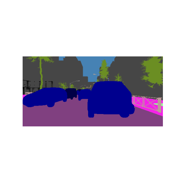
Visualize the same image above but segmented.

tmp_tgt = tgt.masked_fill(tgt == 255, 21)
tgt_masks = tmp_tgt == torch.arange(22, device=tgt.device)[:, None, None]
img_segmented = draw_segmentation_masks(
    img, tgt_masks, alpha=1, colors=datamodule.train.color_palette
)
img_pil = F.to_pil_image(img_segmented)

plt.figure(figsize=(6, 6))
plt.imshow(img_pil)
plt.axis("off")
plt.show()

3. Instantiating the Model

We create the model easily using the blueprint from torch_uncertainty.models.

model = small_unet(
    in_channels=datamodule.num_channels,
    num_classes=datamodule.num_classes,
    bilinear=True,
    dropout_rate=0.1,  # We use dropout to enable MC Dropout later
)

4. Compute class weights to mitigate class inbalance

def enet_weighing(dataloader, num_classes, c=1.02):
    """Computes class weights as described in the ENet paper.

        w_class = 1 / (ln(c + p_class)),

    where c is usually 1.02 and p_class is the propensity score of that
    class:

        propensity_score = freq_class / total_pixels.

    References:
        https://arxiv.org/abs/1606.02147

    Args:
        dataloader (``data.Dataloader``): A data loader to iterate over the
            dataset.
        num_classes (``int``): The number of classes.
        c (``int``, optional): AN additional hyper-parameter which restricts
            the interval of values for the weights. Default: 1.02.
        ignore_indexes (``list``, optional): A list of indexes to ignore
            when computing the weights. Default to `None`.

    """
    class_count = 0
    total = 0
    for _, label in dataloader:
        label = label.cpu()
        # Flatten label
        flat_label = label.flatten()
        flat_label = flat_label[flat_label != 255]
        flat_label = flat_label[flat_label < num_classes]

        # Sum up the number of pixels of each class and the total pixel
        # counts for each label
        class_count += torch.bincount(flat_label, minlength=num_classes)
        total += flat_label.size(0)

    # Compute propensity score and then the weights for each class
    propensity_score = class_count / total

    return 1 / (torch.log(c + propensity_score))


class_weights = enet_weighing(datamodule.val_dataloader(), datamodule.num_classes)
print(class_weights)

tensor([ 4.3817, 19.7927,  3.3011, 48.8031, 36.2141, 33.0049, 47.5130, 48.8560,
        12.4401, 48.0600, 14.4807, 30.8762,  4.7467, 19.3913, 50.4984])

Let’s define the training parameters.

BATCH_SIZE = 10
LEARNING_RATE = 1e-3
WEIGHT_DECAY = 2e-4
LR_DECAY_EPOCHS = 20
LR_DECAY = 0.1
NB_EPOCHS = 1

5. The Loss, the Routine, and the Trainer

# We build the optimizer
optimizer = optim.Adam(model.parameters(), lr=LEARNING_RATE, weight_decay=WEIGHT_DECAY)

# Learning rate decay scheduler
lr_updater = lr_scheduler.StepLR(optimizer, step_size=LR_DECAY_EPOCHS, gamma=LR_DECAY)

# Segmentation Routine
seg_routine = SegmentationRoutine(
    model=model,
    num_classes=datamodule.num_classes,
    loss=torch.nn.CrossEntropyLoss(weight=class_weights),
    optim_recipe={"optimizer": optimizer, "lr_scheduler": lr_updater},
)

trainer = TUTrainer(accelerator="gpu", devices=1, max_epochs=NB_EPOCHS, enable_progress_bar=False)

6. Training the model

trainer.fit(model=seg_routine, datamodule=datamodule)

7. Testing the model

results = trainer.test(datamodule=datamodule, ckpt_path="best")

┏━━━━━━━━━━━━━━┳━━━━━━━━━━━━━━━━━━━━━━━━━━━┓
┃ Test metric  ┃       Segmentation        ┃
┡━━━━━━━━━━━━━━╇━━━━━━━━━━━━━━━━━━━━━━━━━━━┩
│    Brier     │          0.63934          │
│     NLL      │          1.57190          │
│     mAcc     │          26.578%          │
│     mIoU     │          19.289%          │
│    pixAcc    │          63.958%          │
└──────────────┴───────────────────────────┘
┏━━━━━━━━━━━━━━┳━━━━━━━━━━━━━━━━━━━━━━━━━━━┓
┃ Test metric  ┃        Calibration        ┃
┡━━━━━━━━━━━━━━╇━━━━━━━━━━━━━━━━━━━━━━━━━━━┩
│     ECE      │          32.290%          │
│     aECE     │          32.290%          │
└──────────────┴───────────────────────────┘
┏━━━━━━━━━━━━━━┳━━━━━━━━━━━━━━━━━━━━━━━━━━━┓
┃ Test metric  ┃ Selective Classification  ┃
┡━━━━━━━━━━━━━━╇━━━━━━━━━━━━━━━━━━━━━━━━━━━┩
│    AUGRC     │          13.225%          │
│     AURC     │          20.583%          │
│  Cov@5Risk   │           nan%            │
│  Risk@80Cov  │          30.103%          │
└──────────────┴───────────────────────────┘

8. Loading a pre-trained model

Let’s now load a fully trained model to continue this tutorial

model_path = hf_hub_download(repo_id="torch-uncertainty/muad_tutorials", filename="small_unet.pth")
model.load_state_dict(torch.load(model_path))
# Replace the model in the routine
seg_routine.model = model
# Test the model
results = trainer.test(model=seg_routine, datamodule=datamodule)

┏━━━━━━━━━━━━━━┳━━━━━━━━━━━━━━━━━━━━━━━━━━━┓
┃ Test metric  ┃       Segmentation        ┃
┡━━━━━━━━━━━━━━╇━━━━━━━━━━━━━━━━━━━━━━━━━━━┩
│    Brier     │          0.20635          │
│     NLL      │          0.40168          │
│     mAcc     │          68.773%          │
│     mIoU     │          50.739%          │
│    pixAcc    │          85.701%          │
└──────────────┴───────────────────────────┘
┏━━━━━━━━━━━━━━┳━━━━━━━━━━━━━━━━━━━━━━━━━━━┓
┃ Test metric  ┃        Calibration        ┃
┡━━━━━━━━━━━━━━╇━━━━━━━━━━━━━━━━━━━━━━━━━━━┩
│     ECE      │          1.731%           │
│     aECE     │          1.874%           │
└──────────────┴───────────────────────────┘
┏━━━━━━━━━━━━━━┳━━━━━━━━━━━━━━━━━━━━━━━━━━━┓
┃ Test metric  ┃ Selective Classification  ┃
┡━━━━━━━━━━━━━━╇━━━━━━━━━━━━━━━━━━━━━━━━━━━┩
│    AUGRC     │          2.733%           │
│     AURC     │          3.367%           │
│  Cov@5Risk   │          72.133%          │
│  Risk@80Cov  │          7.174%           │
└──────────────┴───────────────────────────┘

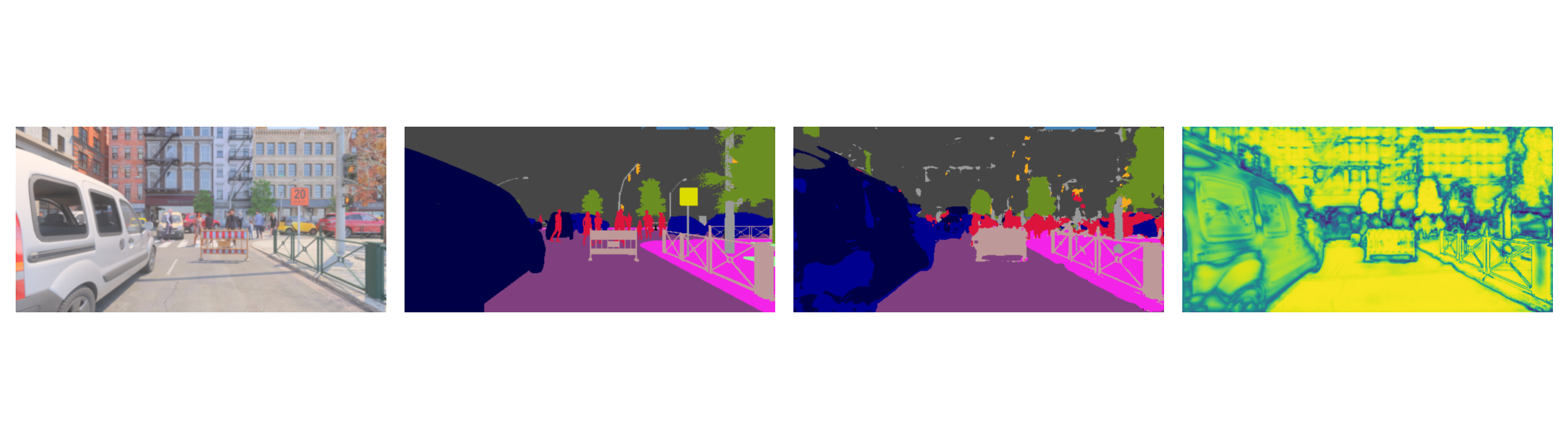
9. Uncertainty evaluations with MCP

Here we will just use as confidence score the Maximum class probability (MCP)

sample_idx = 0
img, target = datamodule.test[sample_idx]

batch_img = img.unsqueeze(0)
batch_target = target.unsqueeze(0)
model.eval()
with torch.no_grad():
    # Forward propagation
    output_probs = model(batch_img).softmax(dim=1)
    # remove the batch dimension
    output_probs = output_probs.squeeze(0)
    confidence, pred = output_probs.max(0)

# Undo normalization on the image and convert to uint8.
img = img * t_muad_std[:, None, None] + t_muad_mean[:, None, None]
img = F.to_dtype(img, torch.uint8, scale=True)

tmp_target = target.masked_fill(target == 255, 21)
target_masks = tmp_target == torch.arange(22, device=target.device)[:, None, None]
img_segmented = draw_segmentation_masks(
    img, target_masks, alpha=1, colors=datamodule.test.color_palette
)

pred_masks = pred == torch.arange(22, device=pred.device)[:, None, None]

pred_img = draw_segmentation_masks(img, pred_masks, alpha=1, colors=datamodule.test.color_palette)


if confidence.ndim == 2:
    confidence = confidence.unsqueeze(0)

img = F.to_pil_image(F.resize(img, 1024))
img_segmented = F.to_pil_image(F.resize(img_segmented, 1024))
pred_img = F.to_pil_image(F.resize(pred_img, 1024))
confidence_img = F.to_pil_image(F.resize(confidence, 1024))


fig, axs = plt.subplots(1, 4, figsize=(25, 7))
images = [img, img_segmented, pred_img, confidence_img]

for ax, im in zip(axs, images, strict=False):
    ax.imshow(im)
    ax.axis("off")

plt.subplots_adjust(left=0.01, right=0.99, top=0.99, bottom=0.01, wspace=0.05)

plt.show()

10. Apply the MC Dropout wrapper

This technique decribed in this paper allow us to have a better confidence score by using the dropout during test time.

# We wrap the model with the MC Dropout wrapper from torch_uncertainty.models.mc_dropout
num_estimators = 10
mc_model = mc_dropout(
    model,
    num_estimators=num_estimators,
    last_layer=False,  # We do not want to apply dropout on the last layer
    on_batch=False,  # To reduce memory usage, we execute the forward passes sequentially
)

seg_routine = SegmentationRoutine(
    model=mc_model,
    num_classes=datamodule.num_classes,
    loss=None,  # No loss needed for testing
)

11. Testing the MC Dropout model

results = trainer.test(model=seg_routine, datamodule=datamodule)

┏━━━━━━━━━━━━━━┳━━━━━━━━━━━━━━━━━━━━━━━━━━━┓
┃ Test metric  ┃       Segmentation        ┃
┡━━━━━━━━━━━━━━╇━━━━━━━━━━━━━━━━━━━━━━━━━━━┩
│    Brier     │          0.20520          │
│     NLL      │          0.40327          │
│     mAcc     │          68.400%          │
│     mIoU     │          50.871%          │
│    pixAcc    │          85.739%          │
└──────────────┴───────────────────────────┘
┏━━━━━━━━━━━━━━┳━━━━━━━━━━━━━━━━━━━━━━━━━━━┓
┃ Test metric  ┃        Calibration        ┃
┡━━━━━━━━━━━━━━╇━━━━━━━━━━━━━━━━━━━━━━━━━━━┩
│     ECE      │          2.792%           │
│     aECE     │          2.792%           │
└──────────────┴───────────────────────────┘
┏━━━━━━━━━━━━━━┳━━━━━━━━━━━━━━━━━━━━━━━━━━━┓
┃ Test metric  ┃ Selective Classification  ┃
┡━━━━━━━━━━━━━━╇━━━━━━━━━━━━━━━━━━━━━━━━━━━┩
│    AUGRC     │          2.680%           │
│     AURC     │          3.288%           │
│  Cov@5Risk   │          72.726%          │
│  Risk@80Cov  │          6.948%           │
└──────────────┴───────────────────────────┘

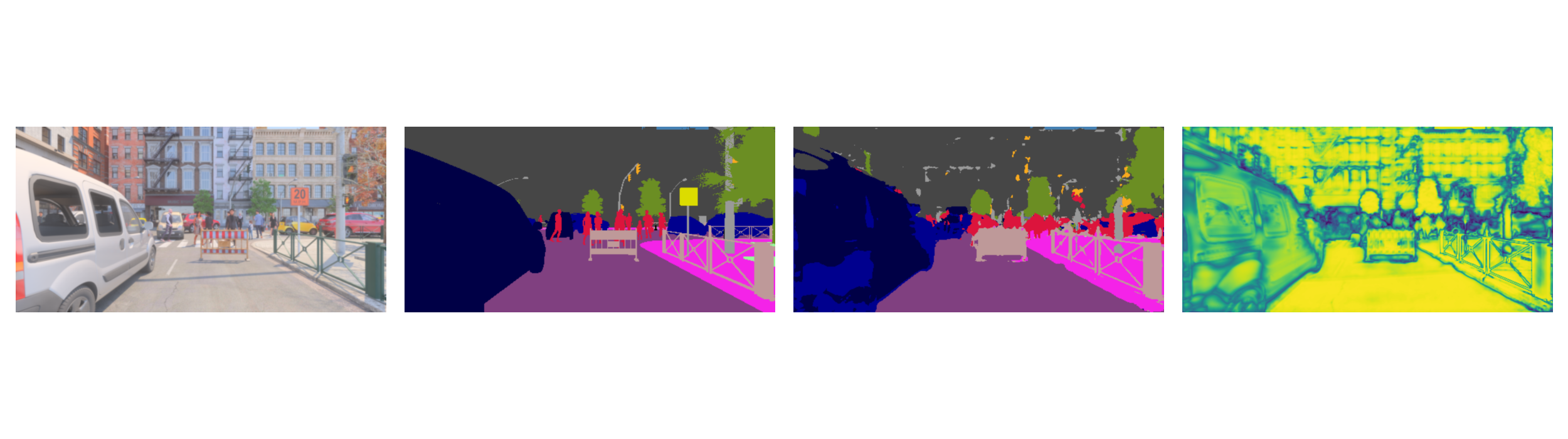
9. Uncertainty evaluations with MCP

Here the confidence score is the Maximum class probability on the averaged probabilities of the different estimators.

sample_idx = 0
img, target = datamodule.test[sample_idx]

batch_img = img.unsqueeze(0)
batch_target = target.unsqueeze(0)
mc_model.eval()
with torch.no_grad():
    # Forward propagation
    output_probs_per_est = mc_model(batch_img).softmax(dim=1)
    output_probs = output_probs_per_est.mean(0)  # Average over the estimators
    # remove the batch dimension
    confidence, pred = output_probs.max(0)

# Undo normalization on the image and convert to uint8.
img = img * t_muad_std[:, None, None] + t_muad_mean[:, None, None]
img = F.to_dtype(img, torch.uint8, scale=True)

tmp_target = target.masked_fill(target == 255, 21)
target_masks = tmp_target == torch.arange(22, device=target.device)[:, None, None]
img_segmented = draw_segmentation_masks(
    img, target_masks, alpha=1, colors=datamodule.test.color_palette
)

pred_masks = pred == torch.arange(22, device=pred.device)[:, None, None]

pred_img = draw_segmentation_masks(img, pred_masks, alpha=1, colors=datamodule.test.color_palette)


if confidence.ndim == 2:
    confidence = confidence.unsqueeze(0)

img = F.to_pil_image(F.resize(img, 1024))
img_segmented = F.to_pil_image(F.resize(img_segmented, 1024))
pred_img = F.to_pil_image(F.resize(pred_img, 1024))
confidence_img = F.to_pil_image(F.resize(confidence, 1024))


fig, axs = plt.subplots(1, 4, figsize=(25, 7))
images = [img, img_segmented, pred_img, confidence_img]

for ax, im in zip(axs, images, strict=False):
    ax.imshow(im)
    ax.axis("off")

plt.subplots_adjust(left=0.01, right=0.99, top=0.99, bottom=0.01, wspace=0.05)

plt.show()