Deep Evidential Regression on a Toy Example

This tutorial provides an introduction to probabilistic regression in TorchUncertainty.

More specifically, we present Deep Evidential Regression (DER) using a practical example. We demonstrate an application of DER by tackling the toy-problem of fitting \(y=x^3\) using a Multi-Layer Perceptron (MLP) neural network model. The output layer of the MLP provides a NormalInverseGamma distribution which is used to optimize the model, through its negative log-likelihood.

DER represents an evidential approach to quantifying epistemic and aleatoric uncertainty in neural network regression models. This method involves introducing prior distributions over the parameters of the Gaussian likelihood function. Then, the MLP model estimates the parameters of this evidential distribution.

Training a MLP with DER using TorchUncertainty models and PyTorch Lightning

In this part, we train a neural network, based on the model and routines already implemented in TU.

1. Loading the utilities

To train a MLP with the DER loss function using TorchUncertainty, we have to load the following modules:

• our TUTrainer

• the model: mlp from torch_uncertainty.models.mlp

• the regression training and evaluation routine from torch_uncertainty.routines

• the evidential objective: the DERLoss from torch_uncertainty.losses. This loss contains the classic NLL loss and a regularization term.

• a dataset that generates samples from a noisy cubic function: Cubic from torch_uncertainty.datasets.regression

We also need to define an optimizer using torch.optim and the neural network utils within torch.nn.

import torch
from lightning import LightningDataModule
from torch import nn, optim

from torch_uncertainty import TUTrainer
from torch_uncertainty.datasets.regression.toy import Cubic
from torch_uncertainty.losses import DERLoss
from torch_uncertainty.models.mlp import mlp
from torch_uncertainty.routines import RegressionRoutine
from torch_uncertainty.utils.distributions import get_dist_class

MAX_EPOCHS = 25
BATCH_SIZE = 64

2. The Optimization Recipe

We use the Adam optimizer with a rate of 4e-3. We increased the learning-rate compared to The original paper to decrease the number of epochs and hence the duration of the experiment.

def optim_regression(
    model: nn.Module,
):
    return optim.Adam(
        model.parameters(),
        lr=4e-3,
        weight_decay=0,
    )

3. Creating the necessary variables

In the following, we create a trainer to train the model, the same synthetic regression datasets as in the original DER paper and the model, a simple MLP with 2 hidden layers of 64 neurons each. Please note that this MLP finishes with a NormalInverseGammaLinear that interpret the outputs of the model as the parameters of a Normal Inverse Gamma distribution.

trainer = TUTrainer(accelerator="gpu", devices=1, max_epochs=MAX_EPOCHS, enable_progress_bar=False)

# dataset
train_ds = Cubic(num_samples=1000)
val_ds = Cubic(num_samples=300)

# datamodule
datamodule = LightningDataModule.from_datasets(
    train_ds, val_dataset=val_ds, test_dataset=val_ds, batch_size=BATCH_SIZE, num_workers=4
)
datamodule.training_task = "regression"

# model
model = mlp(
    in_features=1,
    num_outputs=1,
    hidden_dims=[64, 64],
    dist_family="nig",  # Normal Inverse Gamma
)

4. The Loss and the Training Routine

Next, we need to define the loss to be used during training. To do this, we set the weight of the regularizer of the DER Loss. After that, we define the training routine using the probabilistic regression training routine from torch_uncertainty.routines. In this routine, we provide the model, the DER loss, and the optimization recipe.

loss = DERLoss(reg_weight=1e-2)

routine = RegressionRoutine(
    output_dim=1,
    model=model,
    loss=loss,
    optim_recipe=optim_regression(model),
    dist_family="nig",
)

5. Gathering Everything and Training the Model

Finally, we train the model using the trainer and the regression routine. We also test the model using the same trainer

trainer.fit(model=routine, datamodule=datamodule)
trainer.test(model=routine, datamodule=datamodule)

/home/chocolatine/actions-runner/_work/_tool/Python/3.11.12/x64/lib/python3.11/site-packages/lightning/pytorch/loops/fit_loop.py:310: The number of training batches (16) is smaller than the logging interval Trainer(log_every_n_steps=50). Set a lower value for log_every_n_steps if you want to see logs for the training epoch.
┏━━━━━━━━━━━━━━┳━━━━━━━━━━━━━━━━━━━━━━━━━━━┓
┃ Test metric  ┃        Regression         ┃
┡━━━━━━━━━━━━━━╇━━━━━━━━━━━━━━━━━━━━━━━━━━━┩
│     MAE      │          2.41921          │
│     MSE      │          9.13292          │
│     NLL      │          2.60533          │
│     RMSE     │          3.02207          │
└──────────────┴───────────────────────────┘

[{'test/reg/MAE': 2.4192123413085938, 'test/reg/MSE': 9.132915496826172, 'test/reg/RMSE': 3.022071361541748, 'test/reg/NLL': 2.60532808303833}]

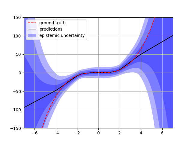
6. Testing the Model

We can now test the model by plotting the predictions and the uncertainty estimates. In this specific case, we can approximately reproduce the figure of the original paper.

import matplotlib.pyplot as plt

with torch.no_grad():
    x = torch.linspace(-7, 7, 1000)
    dist_params = model(x.unsqueeze(-1))
    dists = get_dist_class("nig")(**dist_params)
    means = dists.loc.squeeze(1)
    variances = torch.sqrt(dists.variance_loc).squeeze(1)

fig, ax = plt.subplots(1, 1)
ax.plot(x, x**3, "--r", label="ground truth", zorder=3)
ax.plot(x, means, "-k", label="predictions")
for k in torch.linspace(0, 4, 4):
    ax.fill_between(
        x,
        means - k * variances,
        means + k * variances,
        linewidth=0,
        alpha=0.3,
        edgecolor=None,
        facecolor="blue",
        label="epistemic uncertainty" if not k else None,
    )

plt.gca().set_ylim(-150, 150)
plt.gca().set_xlim(-7, 7)
plt.legend(loc="upper left")
plt.grid()

Reference

• Deep Evidential Regression: Alexander Amini, Wilko Schwarting, Ava Soleimany, & Daniela Rus. NeurIPS 2020.