Note
Go to the end to download the full example code.
Improve Top-label Calibration with Temperature Scaling#
In this tutorial, we use TorchUncertainty to improve the calibration of the top-label predictions and the reliability of the underlying neural network.
This tutorial provides extensive details on how to use the TemperatureScaler class and its derivative, VectorScaler and MatrixScaler. However, please note that this is usually done automatically in the datamodule when setting the postprocess_set to val or test.
Through this tutorial, we also see how to use the datamodules outside any Lightning trainers, and how to use TorchUncertainty’s models.
1. Loading the Utilities#
In this tutorial, we will need:
TorchUncertainty’s Calibration Error metric to compute to evaluate the top-label calibration with ECE and plot the reliability diagrams
the CIFAR-100 datamodule to handle the data
a ResNet 18 as starting model
the temperature scaler to improve the top-label calibration
a utility function to download HF models easily
If you use the classification routine, the plots will be automatically available in the tensorboard logs if you use the log_plots flag.
from torch_uncertainty.datamodules import CIFAR100DataModule
from torch_uncertainty.metrics import CalibrationError
from torch_uncertainty.models.classification import resnet
from torch_uncertainty.post_processing import TemperatureScaler
from torch_uncertainty.utils import load_hf
2. Loading a model from TorchUncertainty’s HF#
To avoid training a model on CIFAR-100 from scratch, we load a model from Hugging Face. This can be done in a one liner:
# Build the model
model = resnet(in_channels=3, num_classes=100, arch=18, style="cifar", conv_bias=False)

# Download the weights (the config is not used here)
weights, config = load_hf("resnet18_c100")

# Load the weights in the pre-built model
model.load_state_dict(weights)
<All keys matched successfully>
3. Setting up the Datamodule and Dataloaders#
To get the dataloader from the datamodule, just call prepare_data, setup, and extract the first element of the test dataloader list. There are more than one element if eval_ood is True: the dataloader of in-distribution data and the dataloader of out-of-distribution data. Otherwise, it is a list of 1 element.
dm = CIFAR100DataModule(root="./data", eval_ood=False, batch_size=32)
dm.prepare_data()
dm.setup("test")
  0%|          | 0.00/169M [00:00<?, ?B/s]
  0%|          | 65.5k/169M [00:00<07:00, 402kB/s]
  0%|          | 229k/169M [00:00<03:40, 764kB/s]
  0%|          | 623k/169M [00:00<01:49, 1.54MB/s]
  1%|          | 1.38M/169M [00:00<00:54, 3.08MB/s]
  1%|          | 2.10M/169M [00:00<00:41, 4.02MB/s]
  3%|▎         | 4.33M/169M [00:00<00:19, 8.54MB/s]
  4%|▎         | 6.09M/169M [00:00<00:15, 10.5MB/s]
  6%|▌         | 10.4M/169M [00:01<00:08, 19.2MB/s]
  9%|▉         | 14.8M/169M [00:01<00:05, 26.3MB/s]
 11%|█         | 18.7M/169M [00:01<00:05, 26.7MB/s]
 14%|█▍        | 23.5M/169M [00:01<00:04, 31.7MB/s]
 17%|█▋        | 28.2M/169M [00:01<00:04, 31.8MB/s]
 19%|█▉        | 32.6M/169M [00:01<00:03, 35.1MB/s]
 22%|██▏       | 36.9M/169M [00:01<00:03, 37.2MB/s]
 24%|██▍       | 40.9M/169M [00:01<00:03, 34.0MB/s]
 27%|██▋       | 45.4M/169M [00:01<00:03, 36.9MB/s]
 29%|██▉       | 49.7M/169M [00:02<00:03, 38.7MB/s]
 32%|███▏      | 53.7M/169M [00:02<00:03, 35.3MB/s]
 34%|███▍      | 58.1M/169M [00:02<00:02, 37.1MB/s]
 37%|███▋      | 62.5M/169M [00:02<00:02, 38.8MB/s]
 39%|███▉      | 66.5M/169M [00:02<00:02, 35.1MB/s]
 41%|████▏     | 70.1M/169M [00:02<00:02, 35.0MB/s]
 44%|████▎     | 73.7M/169M [00:02<00:02, 35.2MB/s]
 46%|████▌     | 77.3M/169M [00:02<00:02, 35.1MB/s]
 48%|████▊     | 80.9M/169M [00:03<00:02, 34.4MB/s]
 50%|█████     | 84.6M/169M [00:03<00:02, 35.2MB/s]
 52%|█████▏    | 88.2M/169M [00:03<00:02, 35.1MB/s]
 54%|█████▍    | 91.8M/169M [00:03<00:02, 34.5MB/s]
 56%|█████▋    | 95.5M/169M [00:03<00:02, 35.2MB/s]
 59%|█████▊    | 99.0M/169M [00:03<00:02, 34.3MB/s]
 61%|██████    | 103M/169M [00:03<00:01, 35.8MB/s]
 63%|██████▎   | 107M/169M [00:03<00:01, 35.1MB/s]
 65%|██████▌   | 111M/169M [00:03<00:01, 34.7MB/s]
 68%|██████▊   | 115M/169M [00:03<00:01, 37.9MB/s]
 70%|███████   | 119M/169M [00:04<00:01, 35.6MB/s]
 73%|███████▎  | 123M/169M [00:04<00:01, 35.0MB/s]
 75%|███████▌  | 127M/169M [00:04<00:01, 37.2MB/s]
 78%|███████▊  | 131M/169M [00:04<00:01, 35.6MB/s]
 80%|███████▉  | 135M/169M [00:04<00:00, 36.4MB/s]
 82%|████████▏ | 139M/169M [00:04<00:00, 35.6MB/s]
 84%|████████▍ | 143M/169M [00:04<00:00, 36.6MB/s]
 87%|████████▋ | 146M/169M [00:04<00:00, 35.4MB/s]
 89%|████████▉ | 150M/169M [00:04<00:00, 34.8MB/s]
 91%|█████████▏| 155M/169M [00:05<00:00, 35.1MB/s]
 94%|█████████▍| 159M/169M [00:05<00:00, 36.0MB/s]
 97%|█████████▋| 164M/169M [00:05<00:00, 36.7MB/s]
100%|██████████| 169M/169M [00:05<00:00, 31.2MB/s]
4. Iterating on the Dataloader and Computing the ECE#
We first split the original test set into a calibration set and a test set for proper evaluation.
When computing the ECE, you need to provide the likelihoods associated with the inputs. To do this, just call PyTorch’s softmax.
To avoid lengthy computations, we restrict the calibration computation to a subset of the test set.
from torch.utils.data import DataLoader, random_split
# Split datasets
dataset = dm.test
cal_dataset, test_dataset = random_split(dataset, [4000, len(dataset) - 4000])
test_dataloader = DataLoader(test_dataset, batch_size=128)
calibration_dataloader = DataLoader(cal_dataset, batch_size=128)
# Initialize the ECE
ece = CalibrationError(task="multiclass", num_classes=100)
# Iterate on the calibration dataloader
for sample, target in test_dataloader:
logits = model(sample)
probs = logits.softmax(-1)
ece.update(probs, target)
# Compute & print the calibration error
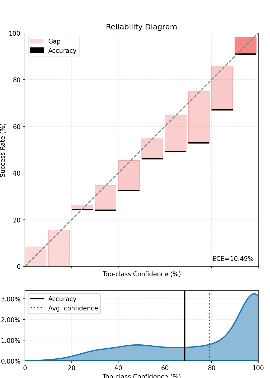
print(f"ECE before scaling - {ece.compute():.3%}.")
ECE before scaling - 11.525%.
We also compute and plot the top-label calibration figure. We see that the model is not well calibrated.
fig, ax = ece.plot()
fig.tight_layout()
fig.show()
5. Fitting the Scaler to Improve the Calibration#
The TemperatureScaler has one parameter that can be used to temper the softmax. We minimize the tempered cross-entropy on a calibration set that we define here as a subset of the test set and containing 1000 data. Look at the code run by TemperatureScaler fit method for more details.
# Fit the scaler on the calibration dataset
scaled_model = TemperatureScaler(model=model)
scaled_model.fit(dataloader=calibration_dataloader)
  0%|          | 0/32 [00:00<?, ?it/s]
  3%|▎         | 1/32 [00:00<00:10,  3.06it/s]
  6%|▋         | 2/32 [00:00<00:09,  3.05it/s]
  9%|▉         | 3/32 [00:00<00:09,  3.05it/s]
 12%|█▎        | 4/32 [00:01<00:09,  3.05it/s]
 16%|█▌        | 5/32 [00:01<00:08,  3.04it/s]
 19%|█▉        | 6/32 [00:01<00:08,  3.04it/s]
 22%|██▏       | 7/32 [00:02<00:08,  3.04it/s]
 25%|██▌       | 8/32 [00:02<00:07,  3.04it/s]
 28%|██▊       | 9/32 [00:02<00:07,  3.04it/s]
 31%|███▏      | 10/32 [00:03<00:07,  3.04it/s]
 34%|███▍      | 11/32 [00:03<00:06,  3.04it/s]
 38%|███▊      | 12/32 [00:03<00:06,  3.04it/s]
 41%|████      | 13/32 [00:04<00:06,  3.04it/s]
 44%|████▍     | 14/32 [00:04<00:05,  3.04it/s]
 47%|████▋     | 15/32 [00:04<00:05,  3.04it/s]
 50%|█████     | 16/32 [00:05<00:05,  3.05it/s]
 53%|█████▎    | 17/32 [00:05<00:04,  3.05it/s]
 56%|█████▋    | 18/32 [00:05<00:04,  3.05it/s]
 59%|█████▉    | 19/32 [00:06<00:04,  3.05it/s]
 62%|██████▎   | 20/32 [00:06<00:03,  3.05it/s]
 66%|██████▌   | 21/32 [00:06<00:03,  3.05it/s]
 69%|██████▉   | 22/32 [00:07<00:03,  3.05it/s]
 72%|███████▏  | 23/32 [00:07<00:02,  3.05it/s]
 75%|███████▌  | 24/32 [00:07<00:02,  3.05it/s]
 78%|███████▊  | 25/32 [00:08<00:02,  3.05it/s]
 81%|████████▏ | 26/32 [00:08<00:01,  3.05it/s]
 84%|████████▍ | 27/32 [00:08<00:01,  3.06it/s]
 88%|████████▊ | 28/32 [00:09<00:01,  3.06it/s]
 91%|█████████ | 29/32 [00:09<00:00,  3.05it/s]
 94%|█████████▍| 30/32 [00:09<00:00,  3.05it/s]
 97%|█████████▋| 31/32 [00:10<00:00,  3.05it/s]
100%|██████████| 32/32 [00:10<00:00,  3.12it/s]
6. Iterating Again to Compute the Improved ECE#
We can directly use the scaler as a calibrated model.
Note that you will need to first reset the ECE metric to avoid mixing the scores of the previous and current iterations.
# Reset the ECE
ece.reset()

# Iterate on the test dataloader
for sample, target in test_dataloader:
    logits = scaled_model(sample)
    probs = logits.softmax(-1)
    ece.update(probs, target)

print(
    f"ECE after scaling - {ece.compute():.3%} with temperature {scaled_model.temperature[0].item():.3}."
)
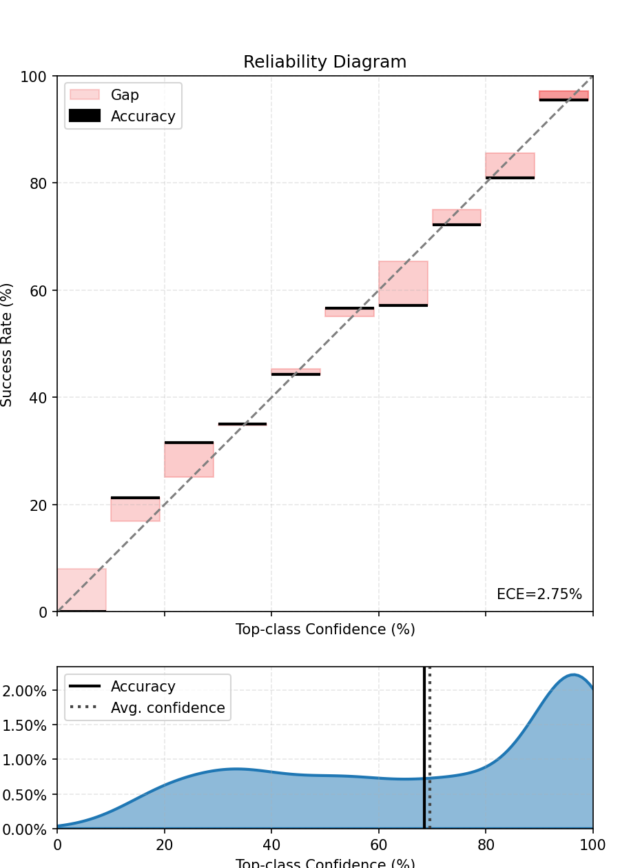
ECE after scaling - 3.769% with temperature 1.37.
We finally compute and plot the scaled top-label calibration figure. We see that the model is now better calibrated. If the temperature is greater than 1, the final model is less confident than before.
fig, ax = ece.plot()
fig.tight_layout()
fig.show()
The top-label calibration should be improved.
7. What about Vector Scaling?#
The VectorScaler has as many parameters as the number of classes to temper the softmax. Instead of a single parameter for all classes, vector scaling fits one temperature for each output class. It can be used just like the TemperatureScaler but we need to specify the number of classes. Can it continue improving the calibration of our model?
from torch_uncertainty.post_processing import VectorScaler

# Fit the scaler on the calibration dataset
scaled_model = VectorScaler(num_classes=100, model=model)
scaled_model.fit(dataloader=calibration_dataloader)

# Reset the ECE
ece.reset()

# Iterate on the test dataloader
for sample, target in test_dataloader:
    logits = scaled_model(sample)
    probs = logits.softmax(-1)
    ece.update(probs, target)

print(
    f"ECE after vector scaling - {ece.compute():.3%} with average temperature {scaled_model.temperature[0].mean():.3}."
)

fig, ax = ece.plot()
fig.tight_layout()
fig.show()
0%| | 0/32 [00:00<?, ?it/s]
3%|▎ | 1/32 [00:00<00:10, 2.86it/s]
6%|▋ | 2/32 [00:00<00:10, 2.84it/s]
9%|▉ | 3/32 [00:01<00:10, 2.83it/s]
12%|█▎ | 4/32 [00:01<00:09, 2.82it/s]
16%|█▌ | 5/32 [00:01<00:09, 2.82it/s]
19%|█▉ | 6/32 [00:02<00:09, 2.81it/s]
22%|██▏ | 7/32 [00:02<00:08, 2.82it/s]
25%|██▌ | 8/32 [00:02<00:08, 2.82it/s]
28%|██▊ | 9/32 [00:03<00:08, 2.82it/s]
31%|███▏ | 10/32 [00:03<00:07, 2.81it/s]
34%|███▍ | 11/32 [00:03<00:07, 2.81it/s]
38%|███▊ | 12/32 [00:04<00:07, 2.81it/s]
41%|████ | 13/32 [00:04<00:06, 2.81it/s]
44%|████▍ | 14/32 [00:04<00:06, 2.81it/s]
47%|████▋ | 15/32 [00:05<00:06, 2.81it/s]
50%|█████ | 16/32 [00:05<00:05, 2.81it/s]
53%|█████▎ | 17/32 [00:06<00:05, 2.81it/s]
56%|█████▋ | 18/32 [00:06<00:04, 2.81it/s]
59%|█████▉ | 19/32 [00:06<00:04, 2.82it/s]
62%|██████▎ | 20/32 [00:07<00:04, 2.82it/s]
66%|██████▌ | 21/32 [00:07<00:03, 2.81it/s]
69%|██████▉ | 22/32 [00:07<00:03, 2.81it/s]
72%|███████▏ | 23/32 [00:08<00:03, 2.82it/s]
75%|███████▌ | 24/32 [00:08<00:02, 2.82it/s]
78%|███████▊ | 25/32 [00:08<00:02, 2.82it/s]
81%|████████▏ | 26/32 [00:09<00:02, 2.82it/s]
84%|████████▍ | 27/32 [00:09<00:01, 2.82it/s]
88%|████████▊ | 28/32 [00:09<00:01, 2.82it/s]
91%|█████████ | 29/32 [00:10<00:01, 2.82it/s]
94%|█████████▍| 30/32 [00:10<00:00, 2.82it/s]
97%|█████████▋| 31/32 [00:11<00:00, 2.82it/s]
100%|██████████| 32/32 [00:11<00:00, 2.89it/s]
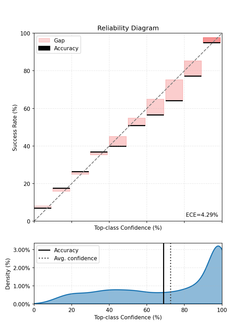
ECE after vector scaling - 4.288% with average temperature 1.35.
It is most likely not the case: we don’t have much data to fit more parameters, and might therefore overfit the calibration set to some extent. Note that the VectorScaler can also change the predictions of the model.
8. What about Matrix Scaling?#
The MatrixScaler has as a number of parameters equal to the square of the number of classes to temper the softmax. It can be used just like the TemperatureScaler but we need to specify the number of classes. Can it continue improving the calibration of our model?
from torch_uncertainty.post_processing import MatrixScaler

# Fit the scaler on the calibration dataset
scaled_model = MatrixScaler(num_classes=100, model=model)
scaled_model.fit(dataloader=calibration_dataloader)

# Reset the ECE
ece.reset()

# Iterate on the test dataloader
for sample, target in test_dataloader:
    logits = scaled_model(sample)
    probs = logits.softmax(-1)
    ece.update(probs, target)

print(
    f"ECE after matrix scaling - {ece.compute():.3%} with average diagonal temperature {scaled_model.temperature[0].diagonal().mean():.3}."
)

fig, ax = ece.plot()
fig.tight_layout()
fig.show()
0%| | 0/32 [00:00<?, ?it/s]
3%|▎ | 1/32 [00:00<00:11, 2.70it/s]
6%|▋ | 2/32 [00:00<00:11, 2.63it/s]
9%|▉ | 3/32 [00:01<00:11, 2.61it/s]
12%|█▎ | 4/32 [00:01<00:10, 2.60it/s]
16%|█▌ | 5/32 [00:01<00:10, 2.60it/s]
19%|█▉ | 6/32 [00:02<00:10, 2.60it/s]
22%|██▏ | 7/32 [00:02<00:09, 2.59it/s]
25%|██▌ | 8/32 [00:03<00:09, 2.59it/s]
28%|██▊ | 9/32 [00:03<00:08, 2.59it/s]
31%|███▏ | 10/32 [00:03<00:08, 2.59it/s]
34%|███▍ | 11/32 [00:04<00:08, 2.59it/s]
38%|███▊ | 12/32 [00:04<00:07, 2.59it/s]
41%|████ | 13/32 [00:05<00:07, 2.59it/s]
44%|████▍ | 14/32 [00:05<00:06, 2.59it/s]
47%|████▋ | 15/32 [00:05<00:06, 2.59it/s]
50%|█████ | 16/32 [00:06<00:06, 2.59it/s]
53%|█████▎ | 17/32 [00:06<00:05, 2.59it/s]
56%|█████▋ | 18/32 [00:06<00:05, 2.59it/s]
59%|█████▉ | 19/32 [00:07<00:05, 2.59it/s]
62%|██████▎ | 20/32 [00:07<00:04, 2.59it/s]
66%|██████▌ | 21/32 [00:08<00:04, 2.60it/s]
69%|██████▉ | 22/32 [00:08<00:03, 2.60it/s]
72%|███████▏ | 23/32 [00:08<00:03, 2.60it/s]
75%|███████▌ | 24/32 [00:09<00:03, 2.59it/s]
78%|███████▊ | 25/32 [00:09<00:02, 2.60it/s]
81%|████████▏ | 26/32 [00:10<00:02, 2.60it/s]
84%|████████▍ | 27/32 [00:10<00:01, 2.60it/s]
88%|████████▊ | 28/32 [00:10<00:01, 2.60it/s]
91%|█████████ | 29/32 [00:11<00:01, 2.60it/s]
94%|█████████▍| 30/32 [00:11<00:00, 2.60it/s]
97%|█████████▋| 31/32 [00:11<00:00, 2.60it/s]
100%|██████████| 32/32 [00:12<00:00, 2.66it/s]
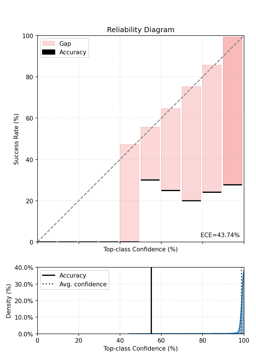
ECE after matrix scaling - 43.743% with average diagonal temperature 0.026.
Here it is a definitive no, we don’t have enough data to fit a MatrixScaler in this case. Note that the MatrixScaler can also change the predictions of the model.
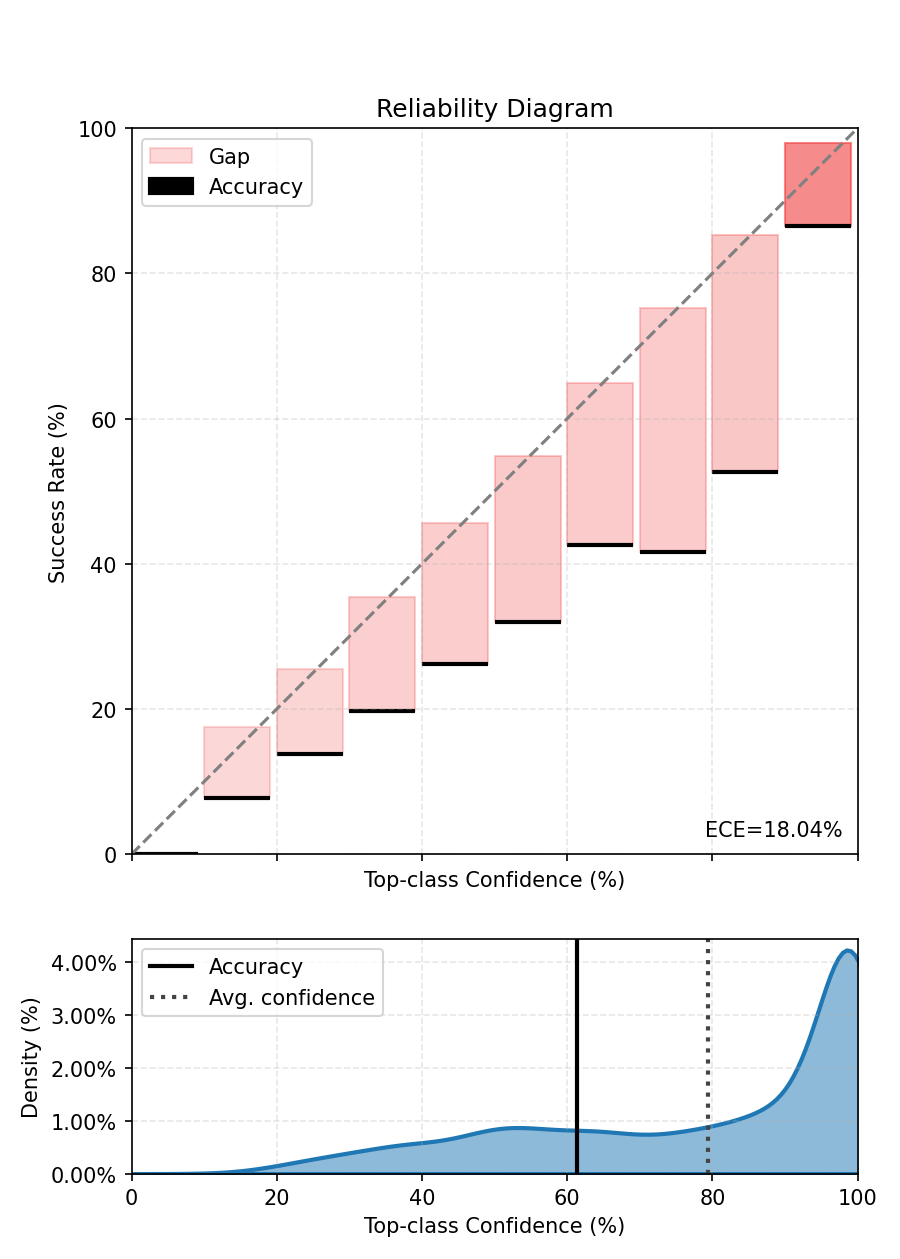
9. Can Dirichlet Calibration help?#
Dirichlet calibration is somewhat similar to matrix scaling, but performs the matrix multiplication directly on the softmax values. Moreover, it includes a regularization mecanism to minimize the L2 norm of the off-diagonal matrix coefficients (lambda_reg) and bias vector (mu_reg).
from torch_uncertainty.post_processing import DirichletScaler

# Fit the scaler on the calibration dataset
scaled_model = DirichletScaler(num_classes=100, model=model, lambda_reg=1, mu_reg=1)
scaled_model.fit(dataloader=calibration_dataloader)

# Reset the ECE
ece.reset()

# Iterate on the test dataloader
for sample, target in test_dataloader:
    logits = scaled_model(sample)
    probs = logits.softmax(-1)
    ece.update(probs, target)

print(f"ECE after Dirichlet calibration - {ece.compute():.3%}.")

fig, ax = ece.plot()
fig.tight_layout()
fig.show()
  0%|          | 0/32 [00:00<?, ?it/s]
  3%|▎         | 1/32 [00:00<00:11,  2.67it/s]
  6%|▋         | 2/32 [00:00<00:11,  2.62it/s]
  9%|▉         | 3/32 [00:01<00:11,  2.60it/s]
 12%|█▎        | 4/32 [00:01<00:10,  2.60it/s]
 16%|█▌        | 5/32 [00:01<00:10,  2.60it/s]
 19%|█▉        | 6/32 [00:02<00:09,  2.61it/s]
 22%|██▏       | 7/32 [00:02<00:09,  2.60it/s]
 25%|██▌       | 8/32 [00:03<00:09,  2.60it/s]
 28%|██▊       | 9/32 [00:03<00:08,  2.60it/s]
 31%|███▏      | 10/32 [00:03<00:08,  2.60it/s]
 34%|███▍      | 11/32 [00:04<00:08,  2.60it/s]
 38%|███▊      | 12/32 [00:04<00:07,  2.59it/s]
 41%|████      | 13/32 [00:04<00:07,  2.60it/s]
 44%|████▍     | 14/32 [00:05<00:06,  2.59it/s]
 47%|████▋     | 15/32 [00:05<00:06,  2.59it/s]
 50%|█████     | 16/32 [00:06<00:06,  2.59it/s]
 53%|█████▎    | 17/32 [00:06<00:05,  2.60it/s]
 56%|█████▋    | 18/32 [00:06<00:05,  2.60it/s]
 59%|█████▉    | 19/32 [00:07<00:05,  2.59it/s]
 62%|██████▎   | 20/32 [00:07<00:04,  2.59it/s]
 66%|██████▌   | 21/32 [00:08<00:04,  2.60it/s]
 69%|██████▉   | 22/32 [00:08<00:03,  2.59it/s]
 72%|███████▏  | 23/32 [00:08<00:03,  2.59it/s]
 75%|███████▌  | 24/32 [00:09<00:03,  2.59it/s]
 78%|███████▊  | 25/32 [00:09<00:02,  2.59it/s]
 81%|████████▏ | 26/32 [00:10<00:02,  2.59it/s]
 84%|████████▍ | 27/32 [00:10<00:01,  2.60it/s]
 88%|████████▊ | 28/32 [00:10<00:01,  2.60it/s]
 91%|█████████ | 29/32 [00:11<00:01,  2.59it/s]
 94%|█████████▍| 30/32 [00:11<00:00,  2.60it/s]
 97%|█████████▋| 31/32 [00:11<00:00,  2.60it/s]
100%|██████████| 32/32 [00:12<00:00,  2.66it/s]
ECE after Dirichlet calibration - 18.044%.
The results are somewhat better than MatrixScaling, but we again do not have enough data to tune the parameters of Dirichlet scaling.
Notes#
Temperature scaling is very efficient when the calibration set is representative of the test set. In this case, we say that the calibration and test set are drawn from the same distribution. However, this may not hold true in real-world cases where dataset shift could happen.
References#
Expected Calibration Error: Naeini, M. P., Cooper, G. F., & Hauskrecht, M. (2015). Obtaining Well Calibrated Probabilities Using Bayesian Binning. In AAAI 2015.
Temperature Scaling: Guo, C., Pleiss, G., Sun, Y., & Weinberger, K. Q. (2017). On calibration of modern neural networks. In ICML 2017.
Total running time of the script: (2 minutes 22.816 seconds)