Packed ensembles Segmentation Tutorial using Muad Dataset

This tutorial demonstrates how to train a segmentation model on the MUAD dataset using TorchUncertainty. MUAD is a synthetic dataset designed for evaluating autonomous driving under diverse uncertainties. It includes 10,413 images across training, validation, and test sets, featuring adverse weather, lighting conditions, and out-of-distribution (OOD) objects. The dataset supports tasks like semantic segmentation, depth estimation, and object detection.

For details and access, visit the MUAD Website.

1. Loading the utilities

First, we load the following utilities from TorchUncertainty:

• the TUTrainer which mostly handles the link with the hardware (accelerators, precision, etc)

• the segmentation training & evaluation routine from torch_uncertainty.routines

• the datamodule handling dataloaders: MUADDataModule from torch_uncertainty.datamodules

import matplotlib.pyplot as plt
import torch
import torchvision.transforms.v2.functional as F
from torch import optim
from torch.optim import lr_scheduler
from torchvision import tv_tensors
from torchvision.transforms import v2
from torchvision.utils import draw_segmentation_masks

from torch_uncertainty import TUTrainer
from torch_uncertainty.datamodules.segmentation import MUADDataModule
from torch_uncertainty.models.segmentation.unet import packed_small_unet
from torch_uncertainty.routines import SegmentationRoutine
from torch_uncertainty.transforms import RepeatTarget

2. Initializing the DataModule

muad_mean = MUADDataModule.mean
muad_std = MUADDataModule.std

train_transform = v2.Compose(
    [
        v2.Resize(size=(256, 512), antialias=True),
        v2.RandomHorizontalFlip(),
        v2.ToDtype(
            dtype={
                tv_tensors.Image: torch.float32,
                tv_tensors.Mask: torch.int64,
                "others": None,
            },
            scale=True,
        ),
        v2.Normalize(mean=[0.485, 0.456, 0.406], std=[0.229, 0.224, 0.225]),
    ]
)

test_transform = v2.Compose(
    [
        v2.Resize(size=(256, 512), antialias=True),
        v2.ToDtype(
            dtype={
                tv_tensors.Image: torch.float32,
                tv_tensors.Mask: torch.int64,
                "others": None,
            },
            scale=True,
        ),
        v2.Normalize(mean=(0.485, 0.456, 0.406), std=(0.229, 0.224, 0.225)),
    ]
)

# datamodule providing the dataloaders to the trainer
datamodule = MUADDataModule(
    root="./data",
    batch_size=10,
    version="small",
    train_transform=train_transform,
    test_transform=test_transform,
    num_workers=4,
)
datamodule.prepare_data()
datamodule.setup("fit")

Visualize a validation input sample (and RGB image)

# Undo normalization on the image and convert to uint8.
img, tgt = datamodule.train[0]
t_muad_mean = torch.tensor(muad_mean, device=img.device)
t_muad_std = torch.tensor(muad_std, device=img.device)
img = img * t_muad_std[:, None, None] + t_muad_mean[:, None, None]
img = F.to_dtype(img, torch.uint8, scale=True)
img_pil = F.to_pil_image(img)

plt.figure(figsize=(6, 6))
plt.imshow(img_pil)
plt.axis("off")
plt.show()

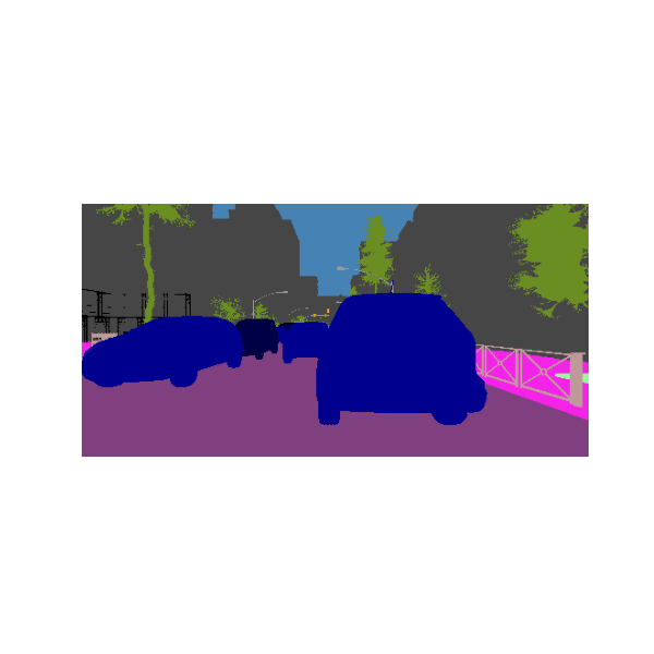
Visualize the same image above but segmented.

tmp_tgt = tgt.masked_fill(tgt == 255, 21)
tgt_masks = tmp_tgt == torch.arange(22, device=tgt.device)[:, None, None]
img_segmented = draw_segmentation_masks(
    img, tgt_masks, alpha=1, colors=datamodule.train.color_palette
)
img_pil = F.to_pil_image(img_segmented)

plt.figure(figsize=(6, 6))
plt.imshow(img_pil)
plt.axis("off")
plt.show()

3. Instantiating the Model

We create the model easily using the blueprint from torch_uncertainty.models.

model = packed_small_unet(
    in_channels=datamodule.num_channels,
    num_classes=datamodule.num_classes,
    alpha=2,
    num_estimators=4,
    gamma=1,
    bilinear=True,
)

4. Compute class weights to mitigate class inbalance

def enet_weighing(dataloader, num_classes, c=1.02):
    """Computes class weights as described in the ENet paper.

        w_class = 1 / (ln(c + p_class)),

    where c is usually 1.02 and p_class is the propensity score of that
    class:

        propensity_score = freq_class / total_pixels.

    References:
        https://arxiv.org/abs/1606.02147

    Args:
        dataloader (``data.Dataloader``): A data loader to iterate over the
            dataset.
        num_classes (``int``): The number of classes.
        c (``int``, optional): AN additional hyper-parameter which restricts
            the interval of values for the weights. Default: 1.02.
        ignore_indexes (``list``, optional): A list of indexes to ignore
            when computing the weights. Default to `None`.

    """
    class_count = 0
    total = 0
    for _, label in dataloader:
        label = label.cpu()
        # Flatten label
        flat_label = label.flatten()
        flat_label = flat_label[flat_label != 255]
        flat_label = flat_label[flat_label < num_classes]

        # Sum up the number of pixels of each class and the total pixel
        # counts for each label
        class_count += torch.bincount(flat_label, minlength=num_classes)
        total += flat_label.size(0)

    # Compute propensity score and then the weights for each class
    propensity_score = class_count / total

    return 1 / (torch.log(c + propensity_score))


class_weights = enet_weighing(datamodule.val_dataloader(), datamodule.num_classes)
print(class_weights)

tensor([ 4.3817, 19.7927,  3.3011, 48.8031, 36.2141, 33.0049, 47.5130, 48.8560,
        12.4401, 48.0600, 14.4807, 30.8762,  4.7467, 19.3913, 50.4984])

Let’s define the training parameters.

BATCH_SIZE = 10
LEARNING_RATE = 1e-3
WEIGHT_DECAY = 2e-4
LR_DECAY_EPOCHS = 20
LR_DECAY = 0.1
NB_EPOCHS = 1
NUM_ESTIMATORS = 4

5. The Loss, the Routine, and the Trainer

# We build the optimizer
optimizer = optim.Adam(
    model.parameters(), lr=LEARNING_RATE * NUM_ESTIMATORS, weight_decay=WEIGHT_DECAY
)

# Learning rate decay scheduler
lr_updater = lr_scheduler.StepLR(optimizer, LR_DECAY_EPOCHS, LR_DECAY)

packed_routine = SegmentationRoutine(
    model=model,
    num_classes=datamodule.num_classes,
    loss=torch.nn.CrossEntropyLoss(weight=class_weights),
    format_batch_fn=RepeatTarget(NUM_ESTIMATORS),  # Repeat the target 4 times for the ensemble
    optim_recipe={"optimizer": optimizer, "lr_scheduler": lr_updater},
)

trainer = TUTrainer(
    accelerator="gpu",
    devices=1,
    max_epochs=NB_EPOCHS,
    enable_progress_bar=False,
    precision="16-mixed",
)

6. Training the model

trainer.fit(model=packed_routine, datamodule=datamodule)

7. Testing the model

results = trainer.test(datamodule=datamodule, ckpt_path="best")

┏━━━━━━━━━━━━━━┳━━━━━━━━━━━━━━━━━━━━━━━━━━━┓
┃ Test metric  ┃       Segmentation        ┃
┡━━━━━━━━━━━━━━╇━━━━━━━━━━━━━━━━━━━━━━━━━━━┩
│    Brier     │          0.67491          │
│     NLL      │          1.61145          │
│     mAcc     │          23.960%          │
│     mIoU     │          12.944%          │
│    pixAcc    │          52.616%          │
└──────────────┴───────────────────────────┘
┏━━━━━━━━━━━━━━┳━━━━━━━━━━━━━━━━━━━━━━━━━━━┓
┃ Test metric  ┃        Calibration        ┃
┡━━━━━━━━━━━━━━╇━━━━━━━━━━━━━━━━━━━━━━━━━━━┩
│     ECE      │          18.491%          │
│     aECE     │          18.658%          │
└──────────────┴───────────────────────────┘
┏━━━━━━━━━━━━━━┳━━━━━━━━━━━━━━━━━━━━━━━━━━━┓
┃ Test metric  ┃ Selective Classification  ┃
┡━━━━━━━━━━━━━━╇━━━━━━━━━━━━━━━━━━━━━━━━━━━┩
│    AUGRC     │          19.938%          │
│     AURC     │          33.967%          │
│  Cov@5Risk   │           nan%            │
│  Risk@80Cov  │          43.517%          │
└──────────────┴───────────────────────────┘

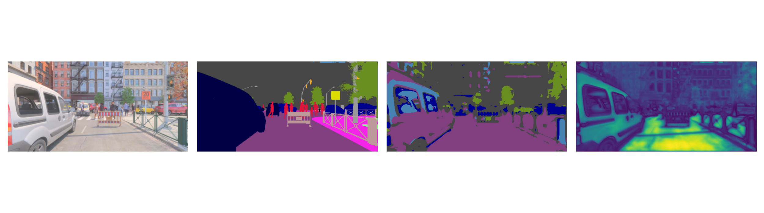
8. Uncertainty evaluations with MCP

Here we will just use as confidence score the Maximum class probability (MCP)

img, target = datamodule.test[0]

batch_img = img.unsqueeze(0)
batch_target = target.unsqueeze(0)
model.eval()
with torch.no_grad():
    # Forward propagation
    outputs = model(batch_img)
    outputs_proba = outputs.softmax(dim=1)
    # average the outputs over the estimators
    outputs_proba = outputs_proba.mean(dim=0)
    # remove the batch dimension
    outputs_proba = outputs_proba.squeeze(0)
    confidence, pred = outputs_proba.max(0)

# Undo normalization on the image and convert to uint8.
mean = torch.tensor([0.485, 0.456, 0.406], device=img.device)
std = torch.tensor([0.229, 0.224, 0.225], device=img.device)
img = img * std[:, None, None] + mean[:, None, None]
img = F.to_dtype(img, torch.uint8, scale=True)

tmp_target = target.masked_fill(target == 255, 21)
target_masks = tmp_target == torch.arange(22, device=target.device)[:, None, None]
img_segmented = draw_segmentation_masks(
    img, target_masks, alpha=1, colors=datamodule.test.color_palette
)

pred_masks = pred == torch.arange(22, device=pred.device)[:, None, None]

pred_img = draw_segmentation_masks(img, pred_masks, alpha=1, colors=datamodule.test.color_palette)


if confidence.ndim == 2:
    confidence = confidence.unsqueeze(0)

img = F.to_pil_image(F.resize(img, 1024))
img_segmented = F.to_pil_image(F.resize(img_segmented, 1024))
pred_img = F.to_pil_image(F.resize(pred_img, 1024))
confidence_img = F.to_pil_image(F.resize(confidence, 1024))


fig, axs = plt.subplots(1, 4, figsize=(25, 7))
images = [img, img_segmented, pred_img, confidence_img]

for ax, im in zip(axs, images, strict=False):
    ax.imshow(im)
    ax.axis("off")

plt.subplots_adjust(left=0.01, right=0.99, top=0.99, bottom=0.01, wspace=0.05)

plt.show()