Conformal Prediction on CIFAR-10 with TorchUncertainty

We evaluate the model’s performance both before and after applying different conformal predictors (THR, APS, RAPS), and visualize how conformal prediction estimates the prediction sets.

We use the pretrained ResNet models we provide on Hugging Face.

import matplotlib.pyplot as plt
import numpy as np
import torch
from huggingface_hub import hf_hub_download

from torch_uncertainty import TUTrainer
from torch_uncertainty.datamodules import CIFAR10DataModule
from torch_uncertainty.models.classification.resnet import resnet
from torch_uncertainty.post_processing import ConformalClsAPS, ConformalClsRAPS, ConformalClsTHR
from torch_uncertainty.routines import ClassificationRoutine

1. Load pretrained model from Hugging Face repository

We use a ResNet18 model trained on CIFAR-10, provided by the TorchUncertainty team

ckpt_path = hf_hub_download(repo_id="torch-uncertainty/resnet18_c10", filename="resnet18_c10.ckpt")
model = resnet(in_channels=3, num_classes=10, arch=18, conv_bias=False, style="cifar")
ckpt = torch.load(ckpt_path, weights_only=True)
model.load_state_dict(ckpt)
model = model.cuda().eval()

2. Load CIFAR-10 Dataset & Define Dataloaders

We set eval_ood to True to evaluate the performance of Conformal scores for detecting out-of-distribution samples. In this case, since we use a model trained on the full training set, we use the test set to as calibration set for the Conformal methods and for its evaluation. This is not a proper way to evaluate the coverage.

BATCH_SIZE = 128

datamodule = CIFAR10DataModule(
    root="./data",
    batch_size=BATCH_SIZE,
    num_workers=8,
    eval_ood=True,
    postprocess_set="test",
)
datamodule.prepare_data()
datamodule.setup()

  0%|          | 0.00/170M [00:00<?, ?B/s]
  0%|          | 65.5k/170M [00:00<07:19, 388kB/s]
  0%|          | 229k/170M [00:00<03:49, 742kB/s]
  0%|          | 623k/170M [00:00<01:54, 1.48MB/s]
  1%|          | 1.38M/170M [00:00<00:56, 3.01MB/s]
  1%|▏         | 2.16M/170M [00:00<00:41, 4.01MB/s]
  3%|▎         | 4.39M/170M [00:00<00:19, 8.41MB/s]
  4%|▎         | 6.39M/170M [00:01<00:15, 10.6MB/s]
  6%|▋         | 10.9M/170M [00:01<00:08, 19.6MB/s]
  9%|▉         | 15.4M/170M [00:01<00:05, 26.5MB/s]
 11%|█▏        | 19.4M/170M [00:01<00:05, 26.4MB/s]
 14%|█▍        | 24.1M/170M [00:01<00:04, 31.5MB/s]
 16%|█▋        | 28.1M/170M [00:01<00:04, 33.9MB/s]
 19%|█▉        | 32.0M/170M [00:01<00:03, 35.2MB/s]
 21%|██        | 35.7M/170M [00:01<00:05, 26.1MB/s]
 24%|██▍       | 41.2M/170M [00:01<00:03, 32.7MB/s]
 27%|██▋       | 45.4M/170M [00:02<00:04, 30.8MB/s]
 29%|██▉       | 49.3M/170M [00:02<00:03, 32.4MB/s]
 31%|███▏      | 53.7M/170M [00:02<00:03, 35.3MB/s]
 34%|███▎      | 57.5M/170M [00:02<00:03, 35.9MB/s]
 36%|███▌      | 61.3M/170M [00:02<00:03, 33.5MB/s]
 38%|███▊      | 65.2M/170M [00:02<00:03, 35.0MB/s]
 40%|████      | 68.9M/170M [00:02<00:02, 35.2MB/s]
 43%|████▎     | 72.8M/170M [00:02<00:02, 36.4MB/s]
 45%|████▍     | 76.5M/170M [00:03<00:02, 33.5MB/s]
 48%|████▊     | 81.1M/170M [00:03<00:02, 35.0MB/s]
 50%|█████     | 85.3M/170M [00:03<00:02, 36.8MB/s]
 52%|█████▏    | 89.0M/170M [00:03<00:02, 34.0MB/s]
 54%|█████▍    | 92.9M/170M [00:03<00:02, 35.1MB/s]
 57%|█████▋    | 96.5M/170M [00:03<00:02, 35.0MB/s]
 59%|█████▉    | 100M/170M [00:03<00:01, 36.3MB/s]
 61%|██████    | 104M/170M [00:03<00:01, 33.7MB/s]
 63%|██████▎   | 108M/170M [00:03<00:01, 35.0MB/s]
 66%|██████▌   | 112M/170M [00:04<00:01, 35.5MB/s]
 68%|██████▊   | 116M/170M [00:04<00:01, 35.1MB/s]
 70%|███████   | 120M/170M [00:04<00:01, 34.0MB/s]
 72%|███████▏  | 124M/170M [00:04<00:01, 35.6MB/s]
 75%|███████▍  | 127M/170M [00:04<00:01, 34.7MB/s]
 77%|███████▋  | 132M/170M [00:04<00:01, 37.7MB/s]
 80%|███████▉  | 136M/170M [00:04<00:01, 34.7MB/s]
 82%|████████▏ | 140M/170M [00:04<00:00, 34.8MB/s]
 84%|████████▍ | 143M/170M [00:04<00:00, 35.1MB/s]
 86%|████████▋ | 147M/170M [00:05<00:00, 34.1MB/s]
 89%|████████▉ | 152M/170M [00:05<00:00, 37.2MB/s]
 91%|█████████▏| 156M/170M [00:05<00:00, 34.6MB/s]
 93%|█████████▎| 159M/170M [00:05<00:00, 34.2MB/s]
 95%|█████████▌| 163M/170M [00:05<00:00, 33.9MB/s]
 97%|█████████▋| 166M/170M [00:05<00:00, 33.9MB/s]
100%|█████████▉| 170M/170M [00:05<00:00, 33.9MB/s]
100%|██████████| 170M/170M [00:05<00:00, 29.9MB/s]

  0%|          | 0.00/64.3M [00:00<?, ?B/s]
  0%|          | 32.8k/64.3M [00:00<04:27, 240kB/s]
  0%|          | 65.5k/64.3M [00:00<05:24, 198kB/s]
  0%|          | 131k/64.3M [00:00<04:19, 247kB/s]
  0%|          | 197k/64.3M [00:00<03:19, 321kB/s]
  0%|          | 295k/64.3M [00:00<02:24, 444kB/s]
  1%|          | 426k/64.3M [00:00<01:46, 602kB/s]
  1%|          | 590k/64.3M [00:01<01:21, 783kB/s]
  1%|▏         | 819k/64.3M [00:01<01:00, 1.05MB/s]
  2%|▏         | 1.11M/64.3M [00:01<00:45, 1.38MB/s]
  2%|▏         | 1.57M/64.3M [00:01<00:31, 1.98MB/s]
  3%|▎         | 2.13M/64.3M [00:01<00:23, 2.61MB/s]
  5%|▍         | 3.01M/64.3M [00:01<00:16, 3.76MB/s]
  6%|▋         | 4.13M/64.3M [00:01<00:11, 5.06MB/s]
  9%|▉         | 5.70M/64.3M [00:02<00:08, 7.00MB/s]
 12%|█▏        | 7.70M/64.3M [00:02<00:06, 9.28MB/s]
 16%|█▌        | 10.1M/64.3M [00:02<00:04, 11.7MB/s]
 19%|█▊        | 12.0M/64.3M [00:02<00:04, 11.5MB/s]
 23%|██▎       | 14.8M/64.3M [00:02<00:03, 14.0MB/s]
 26%|██▌       | 16.6M/64.3M [00:02<00:03, 13.8MB/s]
 29%|██▉       | 18.5M/64.3M [00:02<00:03, 13.7MB/s]
 32%|███▏      | 20.4M/64.3M [00:03<00:03, 13.7MB/s]
 35%|███▍      | 22.3M/64.3M [00:03<00:03, 13.7MB/s]
 38%|███▊      | 24.2M/64.3M [00:03<00:02, 13.8MB/s]
 41%|████      | 26.2M/64.3M [00:03<00:02, 14.0MB/s]
 44%|████▍     | 28.2M/64.3M [00:03<00:02, 14.2MB/s]
 47%|████▋     | 30.2M/64.3M [00:03<00:02, 14.3MB/s]
 50%|█████     | 32.2M/64.3M [00:03<00:02, 14.4MB/s]
 53%|█████▎    | 34.2M/64.3M [00:04<00:02, 14.6MB/s]
 57%|█████▋    | 36.3M/64.3M [00:04<00:01, 14.8MB/s]
 60%|█████▉    | 38.4M/64.3M [00:04<00:01, 14.9MB/s]
 63%|██████▎   | 40.5M/64.3M [00:04<00:01, 15.0MB/s]
 66%|██████▋   | 42.7M/64.3M [00:04<00:01, 15.3MB/s]
 69%|██████▉   | 44.2M/64.3M [00:04<00:01, 13.8MB/s]
 72%|███████▏  | 46.6M/64.3M [00:04<00:01, 15.1MB/s]
 75%|███████▍  | 48.1M/64.3M [00:04<00:01, 13.9MB/s]
 77%|███████▋  | 49.7M/64.3M [00:05<00:01, 13.1MB/s]
 80%|███████▉  | 51.2M/64.3M [00:05<00:01, 12.6MB/s]
 82%|████████▏ | 52.8M/64.3M [00:05<00:00, 12.3MB/s]
 85%|████████▍ | 54.4M/64.3M [00:05<00:00, 12.0MB/s]
 87%|████████▋ | 56.0M/64.3M [00:05<00:00, 11.9MB/s]
 90%|████████▉ | 57.6M/64.3M [00:05<00:00, 11.9MB/s]
 92%|█████████▏| 59.2M/64.3M [00:05<00:00, 11.9MB/s]
 94%|█████████▍| 60.5M/64.3M [00:06<00:00, 10.7MB/s]
 97%|█████████▋| 62.1M/64.3M [00:06<00:00, 11.4MB/s]
 98%|█████████▊| 63.3M/64.3M [00:06<00:00, 10.5MB/s]
100%|██████████| 64.3M/64.3M [00:06<00:00, 10.1MB/s]

3. Define the Lightning Trainer

trainer = TUTrainer(accelerator="gpu", devices=1, max_epochs=5, enable_progress_bar=False)

4. Function to Visualize the Prediction Sets

def visualize_prediction_sets(inputs, labels, confidence_scores, classes, num_examples=5) -> None:
    _, axs = plt.subplots(2, num_examples, figsize=(15, 5))
    for i in range(num_examples):
        ax = axs[0, i]
        img = np.clip(
            inputs[i].permute(1, 2, 0).cpu().numpy() * datamodule.std + datamodule.mean, 0, 1
        )
        ax.imshow(img)
        ax.set_title(f"True: {classes[labels[i]]}")
        ax.axis("off")
        ax = axs[1, i]
        for j in range(len(classes)):
            ax.barh(classes[j], confidence_scores[i, j], color="blue")
        ax.set_xlim(0, 1)
        ax.set_xlabel("Confidence Score")
    plt.tight_layout()
    plt.show()

5. Estimate Prediction Sets with ConformalClsTHR

Using alpha=0.01, we aim for a 1% error rate.

print("[Phase 2]: ConformalClsTHR calibration")
conformal_model = ConformalClsTHR(alpha=0.01, device="cuda")

routine_thr = ClassificationRoutine(
    num_classes=10,
    model=model,
    loss=None,  # No loss needed for evaluation
    eval_ood=True,
    post_processing=conformal_model,
    ood_criterion="post_processing",
)
perf_thr = trainer.test(routine_thr, datamodule=datamodule)

[Phase 2]: ConformalClsTHR calibration

  0%|          | 0/79 [00:00<?, ?it/s]
  1%|▏         | 1/79 [00:00<00:15,  5.10it/s]
 10%|█         | 8/79 [00:00<00:02, 31.20it/s]
 18%|█▊        | 14/79 [00:00<00:01, 40.97it/s]
 25%|██▌       | 20/79 [00:00<00:01, 46.91it/s]
 33%|███▎      | 26/79 [00:00<00:01, 50.63it/s]
 41%|████      | 32/79 [00:00<00:00, 53.13it/s]
 48%|████▊     | 38/79 [00:00<00:00, 54.77it/s]
 56%|█████▌    | 44/79 [00:00<00:00, 55.88it/s]
 63%|██████▎   | 50/79 [00:01<00:00, 56.63it/s]
 71%|███████   | 56/79 [00:01<00:00, 57.13it/s]
 78%|███████▊  | 62/79 [00:01<00:00, 57.50it/s]
 86%|████████▌ | 68/79 [00:01<00:00, 57.79it/s]
 94%|█████████▎| 74/79 [00:01<00:00, 57.98it/s]
100%|██████████| 79/79 [00:01<00:00, 51.56it/s]
┏━━━━━━━━━━━━━━┳━━━━━━━━━━━━━━━━━━━━━━━━━━━┓
┃ Test metric  ┃      Classification       ┃
┡━━━━━━━━━━━━━━╇━━━━━━━━━━━━━━━━━━━━━━━━━━━┩
│     Acc      │          93.380%          │
│    Brier     │          0.10812          │
│   Entropy    │          0.08849          │
│     NLL      │          0.26405          │
└──────────────┴───────────────────────────┘
┏━━━━━━━━━━━━━━┳━━━━━━━━━━━━━━━━━━━━━━━━━━━┓
┃ Test metric  ┃        Calibration        ┃
┡━━━━━━━━━━━━━━╇━━━━━━━━━━━━━━━━━━━━━━━━━━━┩
│     ECE      │          3.537%           │
│     aECE     │          3.499%           │
└──────────────┴───────────────────────────┘
┏━━━━━━━━━━━━━━┳━━━━━━━━━━━━━━━━━━━━━━━━━━━┓
┃ Test metric  ┃       OOD Detection       ┃
┡━━━━━━━━━━━━━━╇━━━━━━━━━━━━━━━━━━━━━━━━━━━┩
│     AUPR     │          86.587%          │
│    AUROC     │          79.260%          │
│   Entropy    │          0.08849          │
│    FPR95     │         100.000%          │
└──────────────┴───────────────────────────┘
┏━━━━━━━━━━━━━━┳━━━━━━━━━━━━━━━━━━━━━━━━━━━┓
┃ Test metric  ┃ Selective Classification  ┃
┡━━━━━━━━━━━━━━╇━━━━━━━━━━━━━━━━━━━━━━━━━━━┩
│    AUGRC     │          0.779%           │
│     AURC     │          0.959%           │
│  Cov@5Risk   │          96.510%          │
│  Risk@80Cov  │          1.200%           │
└──────────────┴───────────────────────────┘
┏━━━━━━━━━━━━━━┳━━━━━━━━━━━━━━━━━━━━━━━━━━━┓
┃ Test metric  ┃      Post-Processing      ┃
┡━━━━━━━━━━━━━━╇━━━━━━━━━━━━━━━━━━━━━━━━━━━┩
│ CoverageRate │          0.99000          │
│   SetSize    │          1.52340          │
└──────────────┴───────────────────────────┘

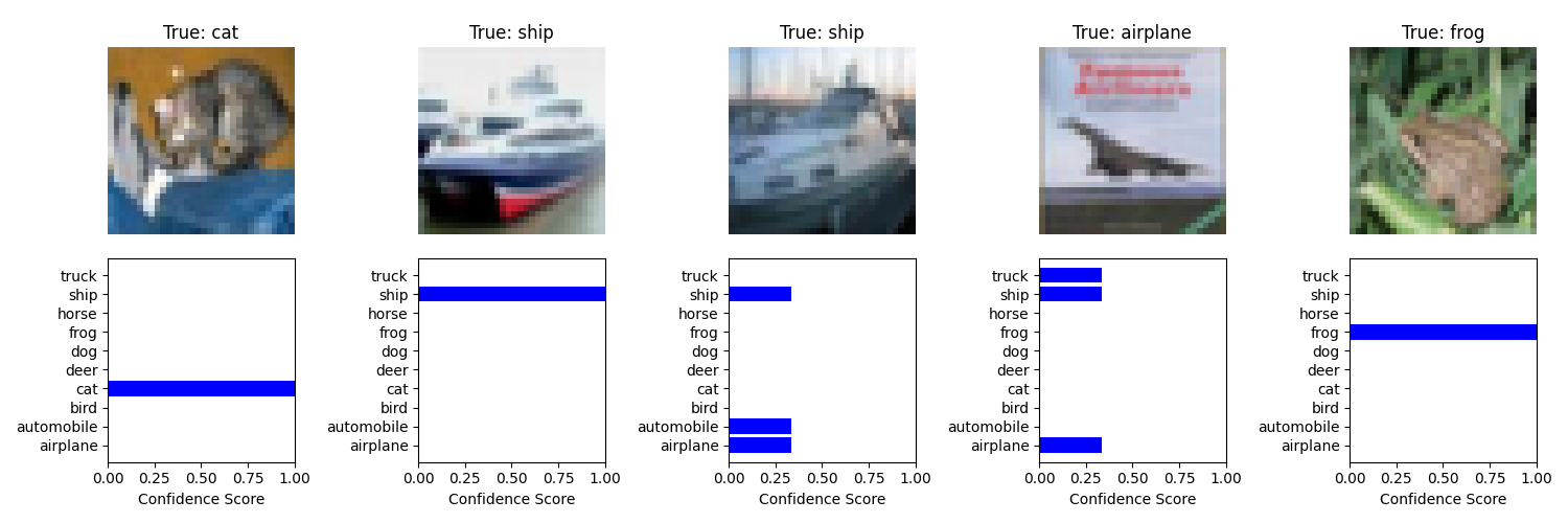
6. Visualization of ConformalClsTHR prediction sets

inputs, labels = next(iter(datamodule.test_dataloader()[0]))

conformal_model.cuda()
confidence_scores = conformal_model.conformal(inputs.cuda())

classes = datamodule.test.classes

visualize_prediction_sets(inputs, labels, confidence_scores[:5].cpu(), classes)

7. Estimate Prediction Sets with ConformalClsAPS

print("[Phase 3]: ConformalClsAPS calibration")
conformal_model = ConformalClsAPS(alpha=0.01, device="cuda", enable_ts=False)

routine_aps = ClassificationRoutine(
    num_classes=10,
    model=model,
    loss=None,  # No loss needed for evaluation
    eval_ood=True,
    post_processing=conformal_model,
    ood_criterion="post_processing",
)
perf_aps = trainer.test(routine_aps, datamodule=datamodule)
conformal_model.cuda()
confidence_scores = conformal_model.conformal(inputs.cuda())
visualize_prediction_sets(inputs, labels, confidence_scores[:5].cpu(), classes)

[Phase 3]: ConformalClsAPS calibration
┏━━━━━━━━━━━━━━┳━━━━━━━━━━━━━━━━━━━━━━━━━━━┓
┃ Test metric  ┃      Classification       ┃
┡━━━━━━━━━━━━━━╇━━━━━━━━━━━━━━━━━━━━━━━━━━━┩
│     Acc      │          93.380%          │
│    Brier     │          0.10812          │
│   Entropy    │          0.08849          │
│     NLL      │          0.26405          │
└──────────────┴───────────────────────────┘
┏━━━━━━━━━━━━━━┳━━━━━━━━━━━━━━━━━━━━━━━━━━━┓
┃ Test metric  ┃        Calibration        ┃
┡━━━━━━━━━━━━━━╇━━━━━━━━━━━━━━━━━━━━━━━━━━━┩
│     ECE      │          3.537%           │
│     aECE     │          3.499%           │
└──────────────┴───────────────────────────┘
┏━━━━━━━━━━━━━━┳━━━━━━━━━━━━━━━━━━━━━━━━━━━┓
┃ Test metric  ┃       OOD Detection       ┃
┡━━━━━━━━━━━━━━╇━━━━━━━━━━━━━━━━━━━━━━━━━━━┩
│     AUPR     │          84.793%          │
│    AUROC     │          77.030%          │
│   Entropy    │          0.08849          │
│    FPR95     │         100.000%          │
└──────────────┴───────────────────────────┘
┏━━━━━━━━━━━━━━┳━━━━━━━━━━━━━━━━━━━━━━━━━━━┓
┃ Test metric  ┃ Selective Classification  ┃
┡━━━━━━━━━━━━━━╇━━━━━━━━━━━━━━━━━━━━━━━━━━━┩
│    AUGRC     │          0.779%           │
│     AURC     │          0.959%           │
│  Cov@5Risk   │          96.510%          │
│  Risk@80Cov  │          1.200%           │
└──────────────┴───────────────────────────┘
┏━━━━━━━━━━━━━━┳━━━━━━━━━━━━━━━━━━━━━━━━━━━┓
┃ Test metric  ┃      Post-Processing      ┃
┡━━━━━━━━━━━━━━╇━━━━━━━━━━━━━━━━━━━━━━━━━━━┩
│ CoverageRate │          0.99120          │
│   SetSize    │          1.79430          │
└──────────────┴───────────────────────────┘

8. Estimate Prediction Sets with ConformalClsRAPS

print("[Phase 4]: ConformalClsRAPS calibration")
conformal_model = ConformalClsRAPS(
    alpha=0.01, regularization_rank=3, penalty=0.002, model=model, device="cuda", enable_ts=False
)

routine_raps = ClassificationRoutine(
    num_classes=10,
    model=model,
    loss=None,  # No loss needed for evaluation
    eval_ood=True,
    post_processing=conformal_model,
    ood_criterion="post_processing",
)
perf_raps = trainer.test(routine_raps, datamodule=datamodule)
conformal_model.cuda()
confidence_scores = conformal_model.conformal(inputs.cuda())
visualize_prediction_sets(inputs, labels, confidence_scores[:5].cpu(), classes)

[Phase 4]: ConformalClsRAPS calibration
┏━━━━━━━━━━━━━━┳━━━━━━━━━━━━━━━━━━━━━━━━━━━┓
┃ Test metric  ┃      Classification       ┃
┡━━━━━━━━━━━━━━╇━━━━━━━━━━━━━━━━━━━━━━━━━━━┩
│     Acc      │          93.380%          │
│    Brier     │          0.10812          │
│   Entropy    │          0.08849          │
│     NLL      │          0.26405          │
└──────────────┴───────────────────────────┘
┏━━━━━━━━━━━━━━┳━━━━━━━━━━━━━━━━━━━━━━━━━━━┓
┃ Test metric  ┃        Calibration        ┃
┡━━━━━━━━━━━━━━╇━━━━━━━━━━━━━━━━━━━━━━━━━━━┩
│     ECE      │          3.537%           │
│     aECE     │          3.499%           │
└──────────────┴───────────────────────────┘
┏━━━━━━━━━━━━━━┳━━━━━━━━━━━━━━━━━━━━━━━━━━━┓
┃ Test metric  ┃       OOD Detection       ┃
┡━━━━━━━━━━━━━━╇━━━━━━━━━━━━━━━━━━━━━━━━━━━┩
│     AUPR     │          85.653%          │
│    AUROC     │          77.694%          │
│   Entropy    │          0.08849          │
│    FPR95     │         100.000%          │
└──────────────┴───────────────────────────┘
┏━━━━━━━━━━━━━━┳━━━━━━━━━━━━━━━━━━━━━━━━━━━┓
┃ Test metric  ┃ Selective Classification  ┃
┡━━━━━━━━━━━━━━╇━━━━━━━━━━━━━━━━━━━━━━━━━━━┩
│    AUGRC     │          0.779%           │
│     AURC     │          0.959%           │
│  Cov@5Risk   │          96.510%          │
│  Risk@80Cov  │          1.200%           │
└──────────────┴───────────────────────────┘
┏━━━━━━━━━━━━━━┳━━━━━━━━━━━━━━━━━━━━━━━━━━━┓
┃ Test metric  ┃      Post-Processing      ┃
┡━━━━━━━━━━━━━━╇━━━━━━━━━━━━━━━━━━━━━━━━━━━┩
│ CoverageRate │          0.99050          │
│   SetSize    │          1.65990          │
└──────────────┴───────────────────────────┘

Summary

In this tutorial, we explored how to apply conformal prediction to a pretrained ResNet on CIFAR-10. We evaluated three methods: Thresholding (THR), Adaptive Prediction Sets (APS), and Regularized APS (RAPS). For each, we calibrated on a validation set, evaluated OOD performance, and visualized prediction sets. You can explore further by adjusting alpha, changing the model, or testing on other datasets.